metabolomics-practical

Metabolomics

MetaboLights is a database for metabolomics data hosted at the European Bioinformatics Institute.

ATP is a metabolite found in many biological processes. The compound can be found in MetaboLights with the identifier MTBLC15422. Under the section Biology the studies are found, with identifiers starting with the prefix MTBLS.

how many human studies found ATP?
in how may other species has this metabolite be found?

MetaboLights follows the ISA framework, where ISA is short for Investigation, Study, and Assay. Following this standard, the information about the study, investigations, and assays are stored in structured data (tabular files in ISATab, and in a hierarchical model in ISAJSON). Additional file may be provided for additional information. For example, MetaboLights uses files that start with the prefix m_ where information about the metabolites are collected.

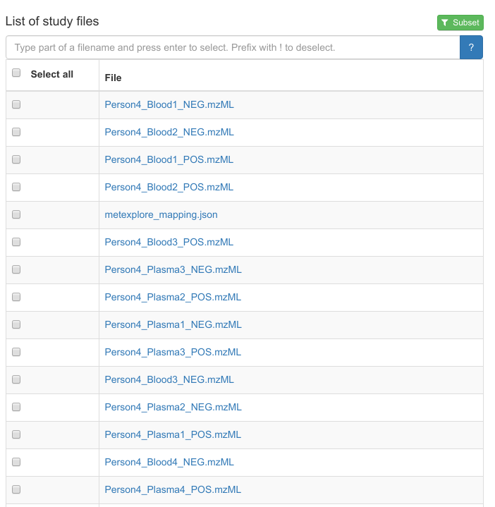
The list of files may look like:

Unexpected similarities

One of the studies where ATP was found is MTBLS88. This study compares human blood samples with Schizosaccharomyces.

Download the m_mtbls88_metabolite_profiling_mass_spectrometry_v2_maf.tsv file from this study. The first few lines look like:

"database_identifier"	"chemical_formula"	"smiles"	"inchi"	"metabolite_identification"	"mass_to_charge"	"fragmentation"	"modifications"	"charge"	"retention_time"	"taxid"	"species"	"database"	"database_version"	"reliability"	"uri"	"search_engine"	"search_engine_score"	"smallmolecule_abundance_sub"	"smallmolecule_abundance_stdev_sub"	"smallmolecule_abundance_std_error_sub"	"Person4_Blood1_POS"	"Person4_Plasma1_POS"	"Person4_RBC1_POS"	"Person4_Blood2_POS"	"Person4_Plasma2_POS"	"Person4_RBC2_POS"	"Person4_Blood3_POS"	"Person4_Plasma3_POS"	"Person4_RBC3_POS"	"Person4_Blood4_POS"	"Person4_Plasma4_POS"	"Person4_RBC4_POS"
"CHEBI:16020"	"C11H15N5O4"	"CN1C=NC2=C(C1=N)N=CN2C3C(C(C(O3)CO)O)O"	"InChI=1S/C11H15N5O4/c1-15-3-14-10-6(9(15)12)13-4-16(10)11-8(19)7(18)5(2-17)20-11/h3-5,7-8,11-12,17-19H,2H2,1H3/t5-,7-,8-,11-/m1/s1"	"1-Methyl-adenosine"	"282.12"	""	"[M+H]+"	"positive"	"11.1"	"NCBITAXON:http://purl.obolibrary.org/obo/NCBITaxon_9606"	"Homo sapiens"	""	""	"5:very good reliability"	""	""	""	""	""	""	"6800000"	"5600000"	"6100000"	"6200000"	"4800000"	"6200000"	"6000000"	"4500000"	"6400000"	"6700000"	"5300000"	"7200000"
"CHEBI:19062"	"C11H15N5O5"	"CN1C(=O)C2=C(N=C1N)N(C=N2)C3C(C(C(O3)CO)O)O"	"InChI=1S/C11H15N5O5/c1-15-9(20)5-8(14-11(15)12)16(3-13-5)10-7(19)6(18)4(2-17)21-10/h3-4,6-7,10,17-19H,2H2,1H3,(H2,12,14)/t4-,6-,7-,10-/m1/s1"	"1-Methyl-guanosine"	"298.115"	""	"[M+H]+"	"positive"	"7.1"	"NCBITAXON:http://purl.obolibrary.org/obo/NCBITaxon_9606"	"Homo sapiens"	""	""	"5:very good reliability"	""	""	""	""	""	""	"190000"	"110000"	"140000"	"220000"	"160000"	"110000"	"210000"	"140000"	"130000"	"160000"	"110000"	"160000"
"CHEBI:84981"	"C6H9NO4-2"	"NC(CCCC([O-])=O)C([O-])=O"	"InChI=1S/C6H11NO4/c7-4(6(10)11)2-1-3-5(8)9/h4H,1-3,7H2,(H,8,9)(H,10,11)/p-2"	"2-Aminoadipate"	"162.076"	""	"[M+H]+"	"positive"	"12.2"	"NCBITAXON:http://purl.obolibrary.org/obo/NCBITaxon_9606"	"Homo sapiens"	""	""	"5:very good reliability"	""	""	""	""	""	""	"1400000"	"1400000"	"1400000"	"1400000"	"1400000"	"1200000"	"1400000"	"1300000"	"1100000"	"1500000"	"1500000"	"1500000"
"CHEBI:17836"	"C7H6NO2-"	"Nc1ccc(cc1)C([O-])=O"	"InChI=1S/C7H7NO2/c8-6-3-1-5(2-4-6)7(9)10/h1-4H,8H2,(H,9,10)/p-1"	"4-Aminobenzoate"	"138.055"	""	"[M+H]+"	"positive"	"7.2"	"NCBITAXON:http://purl.obolibrary.org/obo/NCBITaxon_9606"	"Homo sapiens"	""	""	"5:very good reliability"	""	""	""	""	""	""	"39000"	"39000"	"150000"	"24000"	"84000"	"150000"	"39000"	"76000"	"170000"	"74000"	"110000"	"240000"

Open this file in RStudio Desktop:

mtbls88 = read.table(
  file = "m_mtbls88_metabolite_profiling_mass_spectrometry_v2_maf.tsv",
  header=TRUE
)

how many rows and columns has this file?
why does the 49th data line list two ChEBI identifiers (for C₈H₁₅NO₃)?

The metabolites can be sorted in the order the came of the chromatographic column. This information is given in the retention_time column. We can sort the table with the following command:

mtbls88[ order(mtbls88[,"retention_time"]), ]

what is the compound that came of the column first?
what is the ChEBI identifier of this compound?

Principal Component Analysis

Out discussed during the lecture, we do not need to know the metabolites to do a multivariate analysis of the data. For example, the following R code can be used to run a principal component analysis (PCA):

dataColumns = colnames(mtbls88)[22:33]
data = mtbls88[,dataColumns]
data.pca = prcomp(data, center = TRUE, scale. = TRUE)
biplot(data.pca, scale = 0, cex = .7)

which metabolite is the most descriptive for blood and RBC samples?
what can you tell about the differences between blood, RBC, and plasma?

We can also transpose the matrix, and plot the different samples as points. That allows us to compare the various groups. There are better approaches but a quick go at this can be done with:

data.pca2 = prcomp(t(data), center = TRUE, scale. = TRUE)
colors = c(
  "red",  # blood
  "blue", # plasma
  "green" # RBC
)
plot(data.pca2$x[,1:2], col=colors)

Does the separation of the sample types match your earlier observation?

toc