metabolomics-practical

Pathway Analysis

Continuing from the data set we looked at in the previous section, we first have to define the two sitations we want to compare. Otherwise, we cannot saw which pathways are changed when comparing the two situations. Let’s compare the read blood cell samples with plasma:

rbcColumns = c(
  "Person4_RBC1_POS", "Person4_RBC2_POS",
  "Person4_RBC3_POS", "Person4_RBC4_POS"
)
plasmaColumns = c(
  "Person4_Plasma1_POS", "Person4_Plasma2_POS",
  "Person4_Plasma3_POS", "Person4_Plasma4_POS"
)

Using these two groups, we can calculate log fold changes (logFC) with:

logFC = log2(
  apply(mtbls88[,rbcColumns], 1, function(x) sum(x)) /
  apply(mtbls88[,plasmaColumns], 1, function(x) sum(x))
)
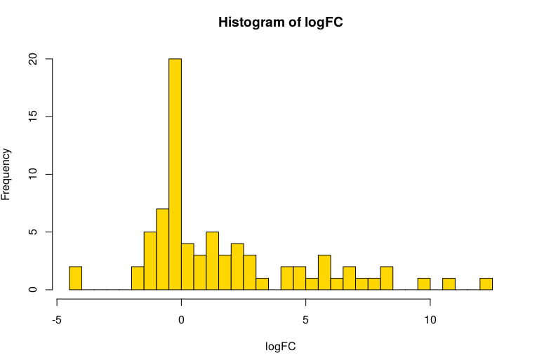
hist(logFC, breaks = 50, col="gold")

The hist() command shows a histogram of of the fold changes:

We are going to use this data in PathVisio (which you may need to install first) and need to export it as a TSV file first. We create a new data matrix, and leave out a few rows:

logFCdata = cbind(
    as.character(mtbls88[,"database_identifier"]),
    logFC
  )[-c(27,47,49,75,77),]
write.table(
  logFCdata, file = "logfc.tsv",
  sep = "\t",
  col.names = c("ChEBI", "logFC"),
  row.names = FALSE, quote = FALSE
)

Loading the fold changes into PathVisio

Following the same approach for pathway analysis with other omics data, we can use this data to find potentially interesting pathways. First, download the metabolite identifier database and open that in PathVisio with Data, Select Metabolite Database.

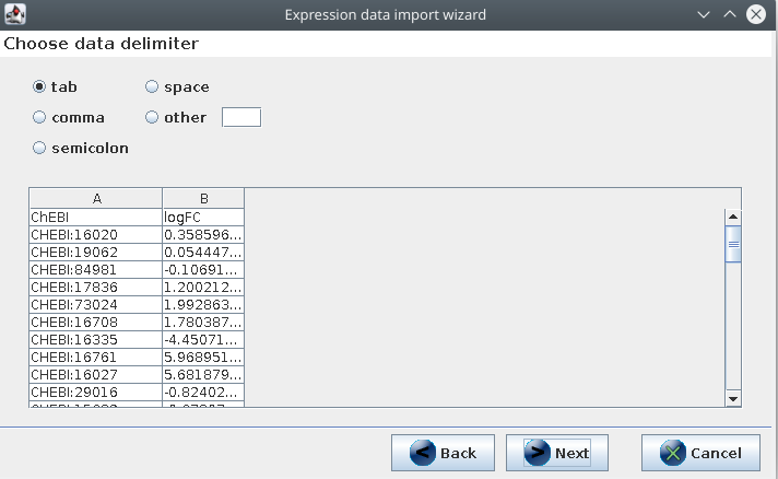
Then, import the logfc.tsv file you created in the previous step into PathVisio with Data, Import expression data. The file is TAB separated:

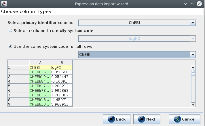
The first CHEBI column has the identifiers, and they are all ChEBI identifiers:

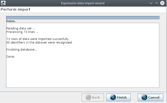
If all went well with loading the metabolite identifier database and importing the expression data, then all 73 data rows should be imported correctly and all identifiers recognized:

Finding pathways with PathVisio

The next step is to download the human pathways and unzip the file locally. Maybe you have them still around from a previous practical. Then downloading them again is not needed.

The pathway analysis goes in exactly the same way as for genes, except that we do not have p-values. The analysis with Data, Statistics... has a simpler equation. The list of metabolites is similar (or use the equation [logFC] < -0.2 OR [logFC] > 0.2):

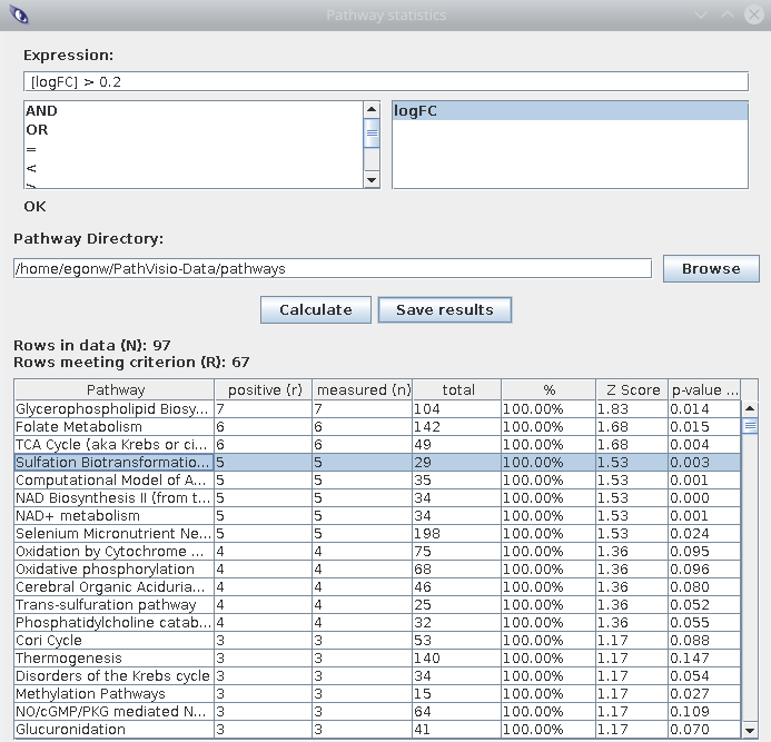
After calculating the enrichment, make sure pathways have non-zero values in the positives and measured columnd. The second is the number of metabolites in this pathway for which the experimental data has fold changes. The positives is the number of measured metabolites that meet the expression.

Make sure to open the pathway to see what it looks like. For example, here is the experimental data mapped onto WP692:

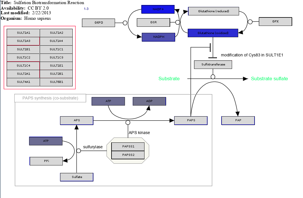
would you expect to see experimental data for reduced glutathion?
if we look at the first few pathways, with the general patterns do we see?

General thoughts

are 73 metabolites enough to do pathway analysis?

Open the TCA cycle pathway in PathVisio and click the NAD on the right side, and open the Backpage sidepanel in PathVisio, like this:

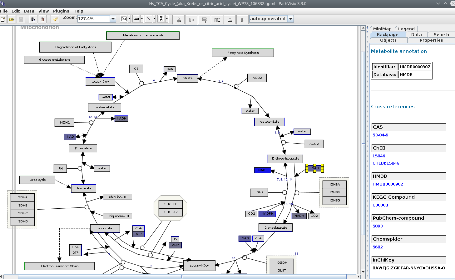
At the top we can see that the NAD node in the pathway is annotated with an HMDB identifier. PathVisio used the BridgeDb metabolite identifier mapping database to recognize that the HMDB identifier in the pathway and the ChEBI identifier for the experimental data actually are about the same metabolite. Then:

thinking about the previous sections of this practical and the lecture, what other things could we do to improve this analysis?

toc